BLUEBikes, a public bike share system based in the US, collect lots of data around their riders’ activity. The best (and most fun) way to analyze this is using geospatial data visualization. It means you can easily answer questions like: Which days of the week do most people cycle on? Which bike stations are the most popular? How far and wide do they travel, and how fast can they pedal?
We bootstrapped RedwoodJS to ReGraph, our graph visualization toolkit for React developers, to build an app that charts BLUEBikes customer activity across Boston, Massachusetts. It took us no longer than a bike ride from Harvard University to South Boston Library and back. To find out how we did it, grab your helmet and get ready to follow a whole month of bike rides.
Creating a geospatial data visualization using RedwoodJS
The RedwoodJS ‘getting started’ guide makes it easy to begin building our app. You can find out about the prerequisites in this excellent RedwoodJS video.
In this tutorial we’ll use:
First, we use yarn’s create command to bootstrap the application:
yarn create redwood-app redwood-app
Now that we’ve created the basic app, we check that everything’s worked correctly by running:
cd redwood-app
yarn rw dev
This starts both the front end and back end, and opens RedwoodJS’s default welcome page:
Creating our first page & adding a ReGraph chart
To add ReGraph to our application and install Leaflet, we run:
cp ~/Downloads/regraph-3.6.3+perpetual-2025-03-20.tgz .
yarn add ./regraph-3.6.3+perpetual-2025-03-20.tgz [email protected]
Now we create our new page:
yarn rw g page Index / --no-tests --no-stories
This creates a new file and directory at web/src/pages/IndexPage/IndexPage.js, and replaces the default welcome page.
We’ll import the Chart component from the ReGraph package, and render it from the IndexPage function. We’ll also replace the contents of the web/src/pages/IndexPage/IndexPage.js with:
import { Link, routes } from '@redwoodjs/router'
import { MetaTags } from '@redwoodjs/web'
import { Chart } from 'regraph'

const IndexPage = () => {
  return (
	<>
  	<MetaTags title="Index" description="Index page" />

  	<h1>IndexPage</h1>
  	<p>
    	Find me in <code>./web/src/pages/IndexPage/IndexPage.js</code>
  	</p>
  	<p>
    	My default route is named <code>index</code>, link to me with
    	<Link to={routes.index()}>Index</Link>`
  	</p>

  	<Chart items={{ a: { label: { text: 'Hello from RedwoodJS' } } }} style={{ height: 500 }} />
	</>
  )
}

export default IndexPage
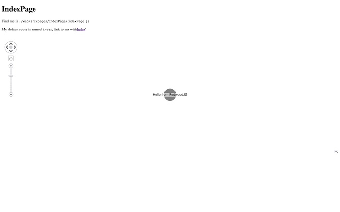
Refresh the page to see our first chart:
What data are we working with?
The data from BLUEBikes relates to trips between stations. We’re interested in:
- the dates of each journey
- where each bike ride started and ended
- how long each trip lasted.
Creating the database schema
Redwood uses Prisma as a database abstraction layer. We’re using a SQLite database here, but you can also connect to other SQL or NoSQL databases such as PostgresSQL or MongoDB – all of our toolkits are database agnostic.
To define our schema we edit the file api/db/schema.prisma and create models for Station and Trip:
model Station {
  id   	String  @id
  name 	String
  lat  	Float?
  lng  	Float?
  ends 	Trip[]  @relation("ends")
  starts   Trip[]  @relation("starts")
}

model Trip {
  id        String   @id @default(uuid())
  endId     String
  startId   String
  startTime DateTime?
  duration  Int
  end       Station  @relation("ends", fields: [endId], references: [id])
  start     Station  @relation("starts", fields: [startId], references: [id])
}
Notice how the Station model has fields for id, latitude and longitude, and the name of the trip.
Prisma requires ids for trips, but BLUEBikes data doesn’t assign them, so you can see from the code that our trip model includes an id field that will automatically be filled with a UUID.
Prisma also needs us to assign two relations to each model: starts and ends. These connect each trip to its start and end station.
With the schema.prima file updated we’ll run:
yarn rw prisma migrate dev
This creates (or updates) our SQLite database, giving us a Station and Trips table. Prisma keeps our data consistent by creating indexes and foreign keys automatically.
Loading data into the database
There are various ways to load the data, but we’ll take the opportunity to try out RedwoodJS’s data migrations feature.
When we created the database schema, Prisma applied foreign key constraints to the Trips table for the startId and endId. That means we need to load the Stations data first, so that the Trips data can reference the corresponding Stations.
We download and unpack 202203-bluebikes-tripdata.zip, which contains a complete csv file of data on all trips taken in March 2022.
Next we install the Data Migrations feature by running this command from the root of the project:
yarn rw data-migrate install
yarn rw prisma migrate dev
We’ll also install the csv-parse and date-fns packages as dev dependencies in the api package of our app:
cd api/
yarn add -D csv-parse date-fns
Next, from the root of the project, we create a migration with the name “seed-data” by running:
yarn rw generate dataMigration seed-data
This will auto-generate a filename that includes the date and time you ran the migration: ./api/db/dataMigrations/20220520082149-seed-data.js
Now we create a directory in api/db/dataMigrations with the same name as the file (in this case, it’s “20220520082149-seed-data”) and move the csv file into it:
mkdir ./api/db/dataMigrations/20220520082149-seed-data/
mv ~/Downloads/202203-bluebikes-tripdata.csv ./api/db/dataMigrations/20220520082149-seed-data/
With the data in place, we can write our migration.
First we’ll extract the csv data we need: a list of all the stations that BLUEBikes customers have visited, and all the trip data we’re interested in.
Now we’ll add the station data to the database, followed by the trip data:
import * as fs from 'fs'
import * as path from 'path'
import * as process from 'process'
import * as csvParse from 'csv-parse'
import * as dateFns from 'date-fns'

const MIGRATION_NAME = path.basename(__filename, '.js')
const DATA_FILE = path.resolve(__dirname, MIGRATION_NAME, '202203-bluebikes-tripdata.csv')

const REFERENCE_DATE = new Date()

export default async ({ db }) => {
  const parser = csvParse.parse({ columns: true })
  const stationsDict = {}
  const trips = []
  parser.on('readable', () => {
	let record

	while ((record = parser.read()) !== null) {
  		const start = {
    	id: record['start station id'],
    	lat: parseFloat(record['start station latitude']),
    	lng: parseFloat(record['start station longitude']),
    	name: record['start station name'],
  		}
  	const end = {
    	id: record['end station id'],
    	lat: parseFloat(record['end station latitude']),
    	lng: parseFloat(record['end station longitude']),
    	name: record['end station name'],
  	}
  	const trip = {
    	duration: parseInt(record.tripduration, 10),
    	endId: end.id,
    	startId: start.id,
    	startTime: dateFns.parse(record.starttime, 'yyyy-MM-dd HH:mm:ss.SSSS', REFERENCE_DATE),
  	}

  	stationsDict[start.id] = start
  	stationsDict[end.id] = end
  	trips.push(trip)
	}
  })

  fs.createReadStream(DATA_FILE).pipe(parser)
  // Wait for the file to completely read
  await new Promise((resolve) => parser.on('end', resolve))

  // Import the stations
  const stations = Object.values(stationsDict)
  for (let i = 0; i < stations.length; i++) {
	await db.station.create({ data: stations[i] })
  	process.stdout.write(`rImported ${i} stations`)
  }
  process.stdout.write(`n`)

  // Import the trips
  for (let i = 0; i < trips.length; i++) {
	await db.trip.create({ data: trips[i] })
  	process.stdout.write(`rImported ${i} trips`)
  }
  process.stdout.write(`n`)
}
And then start the migration using this command:
yarn rw data-migrate up
The migration might take a while to run, because we’re importing 388 stations and a whopping 182421 trips into the database. The perfect opportunity for you to take a quick bike ride around the block.
Exploring the database
Once the migration is complete, we can explore our data with Prisma Studio, the visual database editor that comes with RedwoodJS. To start it, we run:
yarn rw prisma studio
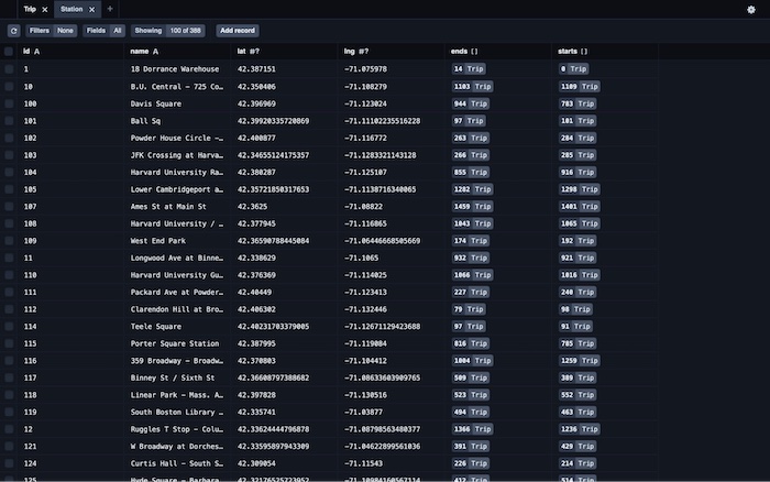
Here’s how our Station table looks:
Note: If you’d prefer to use a pure database tool, you can use a SQLite client such as sqlite3 or DB Browser for SQLite. The database file is located at api/db/dev.db.
Loading the data into the application
With our back end work complete, we’ll make our data accessible from the front end. First, we’ll generate the GraphQL schema (not to be confused with the Prisma schema), along with services that tell RedwoodJS how to load data from the database.
From our project’s root, we run:
yarn rw g sdl Station --no-crud --no-tests
yarn rw g sdl Trip --no-crud --no-tests
This generates the following files:
- stations.sdl.js
- trips.sdl.js, in api/src/graphql
- api/src/services/stations/stations.js
- api/src/services/trips/trips.js
We’ll also generate a Cell to access the data, by running:
yarn rw g cell Stations --no-tests --no-stories
This creates a file named web/src/components/StationsCell/StationsCell.js.
After the cell is generated, we replace the contents of the IndexPage.js file with:
import { MetaTags } from '@redwoodjs/web'
import StationsCell from 'src/components/StationsCell'

const IndexPage = () => {
  return (
	<>
  	<MetaTags title="Index" description="Index page" />

  	<StationsCell />
	</>
  )
}

export default IndexPage
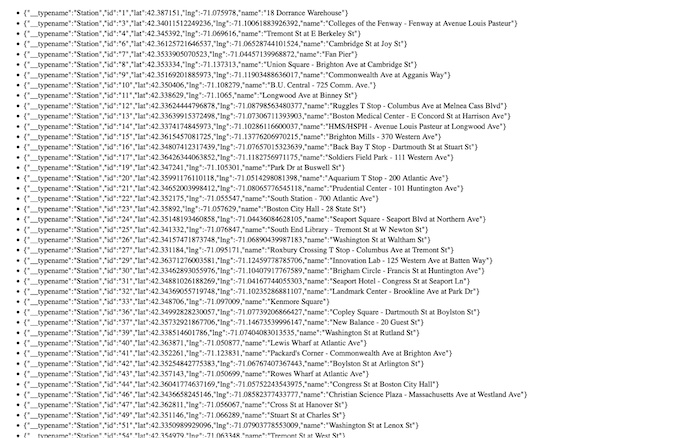
This generates a complete list of station ids, displayed in our browser:

That’s a good start, but our geospatial data visualization needs to show the names and locations of each station. We’ll add those properties to the stations field, in the QUERY defined at the top of StationsCell.js-file:
export const QUERY = gql`
  query StationsQuery {
	stations {
  	id
  	lat
  	lng
  	name
	}
  }
`
The page automatically refreshes with the additional info:
Bringing the data to life
Now it’s time to import the Chart component, along with Leaflet. At the top of the StationsCell.js file, we add:
import {Chart} from 'regraph';
import 'leaflet/dist/leaflet';
import 'leaflet/dist/leaflet.css';
Next we’ll update the Success function in the file, so that it renders a Chart instead of a list. To do this, we take the stations array passed into the Success function and convert it into a ReGraph items object. The methods we need to make this happen are Object.fromEntries and Array#map:
export const Success = ({ stations, trips }) => {
  const nodes = Object.fromEntries(
	stations.map(({ id, lat, lng, name }) => [
  	id,
  	{
    	coordinates: { lat, lng },
    	label: { text: name },
    	color: '#1d428a'
  	},
	])
  )
  return <Chart style={{ height: '100vh' }} map={true} items={nodes} />
}
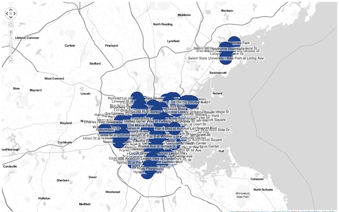
Now things are taking shape – we’ve got a geospatial data visualization showing the locations of all 388 stations:
Joining the dots
It would be easy to load all the trips from the back end and display them on our chart. But if you think of the sheer number of links that would create – things would get messy.
Instead of displaying 180k individual links, let’s aggregate them. The journeys between any two stations will appear as a single link. For a real application, it’s best to take the time to do this in the GraphQL endpoint, which reduces your loading time. However, for this demo we’ll keep things simple and complete the process in the front end.
First we update the QUERY to include the trips field:
export const QUERY = gql`
  query StationsQuery {
	stations {
  	id
  	lat
  	lng
  	name
	}
	trips {
  	endId
  	startId
	}
  }
`
Next we update the Success function so that it aggregates the trips and visualizes them on the map.
export const Success = ({ stations, trips }) => {
  const nodes = Object.fromEntries(
	stations.map(({ id, lat, lng, name }) => [
  	id,
  	{
    	coordinates: { lat, lng },
    	label: { text: name },
    	color: '#1d428a'
  	},
	])
  )
  const links = {}
  trips.forEach(({ startId, endId }) => {
	const id = `${startId}-${endId}`
	if (!(id in links)) {
  		links[id] = { id1: startId, id2: endId, end2: { arrow: true }, color: '#2ca3e1' }
	}
  })
  return <Chart style={{ height: '100vh' }} map={true} items={{ ...nodes, ...links }} />
}
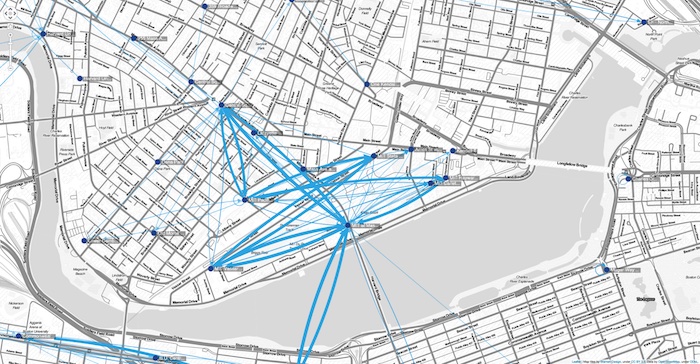
Now the trips between stations are represented by blue arrows. We’ve customized the links so that thicker arrows show journeys that were used more often. If we wanted to, we could use ReGraph’s filtering function to narrow down to the most popular stations – for instance, the stations that were visited by a BLUEBike customer at least 80 times.
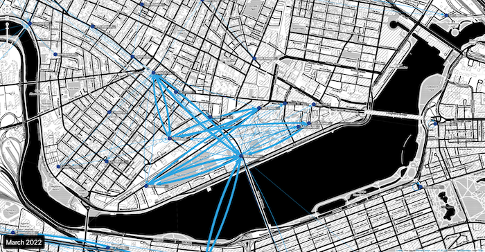
Taking it further
We’ve created a very simple geospatial data visualization, but it doesn’t have to stop here. In the example above we’ve enhanced the map with Toner tiles by Stamen Design. RedwoodJS integrates well with other libraries, too – in the example below we’ve customized the UI with TailWind CSS. Check out our Tailwind CSS tutorial to find out how that might look for your application.
RedwoodJS’s powerful back end allows us to build data-heavy applications quickly, and ReGraph has the high performance needed to keep pace. We’ve shown some of the features that make our toolkit so powerful, but there’s much more to explore. We could develop our application further to show trip and station data gathered across the whole state, use the time bar to filter journeys by date, or use graph analytics to dig into the detail further.
Try MapWeave
If you want to take your geospatial data visualization to the next level, try MapWeave. It comes with expert support, docs, inspirational demos and a smooth DevEx, plus easy integration with our other SDKs.
Share: