How to visualize a DBpedia knowledge graph

Are you a music expert? Do you know your punk from your post-punk? If you don’t, you’ll probably look it up in the world’s biggest knowledge graph: Google. And the top search results will most likely be from another giant in the knowledge graph world: Wikipedia. This developer tutorial shows how we built a knowledge graph visualization tool, using Wikipedia articles to understand the evolution of music. Using SPARQL and RDF Triples to query the database, we’ll show how easy it is to bring DBpedia knowledge graph data to life using our toolkit technology.

To follow the visualization steps, you’ll need access to KeyLines (for JavaScript developers) or ReGraph (for React developers). Not already using our toolkit technology? Simply request a free trial.

What is a knowledge graph?

Knowledge graphs were around long before Google launched theirs back in 2012. There’s an ongoing debate around creating a clear definition, particularly amongst the Web Semantic community, but here are some common characteristics:

• Size – they’re large networks of connected, real-world entities
• Ontology – they feature semantic modeling of knowledge: think of it as a dictionary of descriptive terms we can use to link things
• Integration – they collect information from a variety of external sources

Learn more about visualizing knowledge graphs.

What is DBpedia?

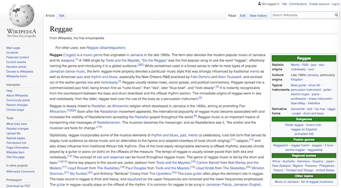
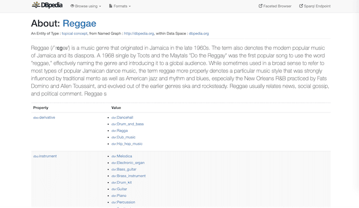
DBpedia is like a machine-readable version of Wikipedia. It’s a huge database built upon structured information found in Wikipedia articles, and has a robot that parses those articles and stores them in a ‘Semantic Web’ format.

This is great for querying the connections between things.

Defining SPARQL and RDF Triples

SPARQL is a query language based on Semantic Web standards from W3C. It’s for querying the Resource Description Framework (RDF) – a data model that describes information as triples of subjects, predicates and objects:

• A subject is the resource being described in our triple
• A predicate defines the relationship within the triple
• An object is something related to the subject, via the predicate

We already use the subject-predicate-object terminology in spoken languages to describe the three components required to form a sentence. This makes RDF triples a logical format for describing a resource:

• Subject: A band
• Predicate: Has
• Object: A genre

SPARQL and ontologies

We know that SPARQL queries run against semantics-based data or ontologies. Let’s look at the ontologies in our DBpedia knowledge graph data.

The DBpedia resource for The Clash has a genre defined as:

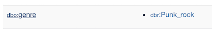
DBpedia stores this a machine representation of this:

< http://dbpedia.org/resource/The_Clash >
< http://dbpedia.org/property/genre >
< http://dbpedia.org/resource/Punk_rock >

Here we’re using 2 ontologies: dbpedia.org/resource and dbpedia.org/property. They’re great because they let us define commonalities between information. We can say that data is linked to other data if they share any of a subject/predicate/object combined with the same ontology.

How to write a SPARQL query for DBpedia

With this knowledge, let’s write our first SPARQL query to run on the live DBpedia SPARQL endpoint.

This is a great place to test your SPARQL skills: http://dbpedia.org/sparql.

Let’s try the following SPARQL query:

PREFIX dbo: <http://dbpedia.org/ontology/>
PREFIX dbr: <http://dbpedia.org/resource/>
PREFIX foaf: <http://xmlns.com/foaf/0.1/>

SELECT ?label, ?band
WHERE {
  ?band dbo:genre dbr:Punk_rock .
  ?band foaf:name ?label .
  FILTER (LANG(?label) = 'en')
}

There are four components to this query:

• The PREFIX at the top – defines the list of ontologies we use in the query.
• The SELECT statement – defines the variables we want to select (these can be any node in the RDF dataset).
• The WHERE clause – which in this case defines a band as something with a genre which is punk_rock. At this stage, we are also saying the label is the name of the band.
• Finally, we apply a filter to show only labels in the English language.

When we click ‘Run Query’, we get a huge table of every punk rock band found on Wikipedia:

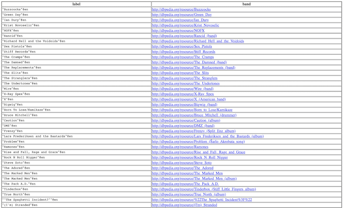
The DBpedia knowledge graph data is not easy to analyze in this format. We need to bring it to life by visualizing it using our toolkit technology. Our products give you the power to quickly build your own knowledge graph visualization tool.

Building a DBpedia knowledge graph visualization

For every music genre we’ll create a parent/child structure – perfect for knowledge graphs! We’ll do this with ‘stylisticOrigin’ and ‘derivative’ properties:

• stylisticOrigin – parent genres that influenced other genres.
• derivative – child genres that were inspired by, or branched from, other genres.

Let’s write our SPARQL query:

PREFIX rdfs: <http://www.w3.org/2000/01/rdf-schema#>
PREFIX dbpedia: <http://dbpedia.org/property/>

SELECT ?label, ?genre, ?origins, ?derivatives, ?decade WHERE {
    { ?genre a dbo:MusicGenre } .
    { ?genre rdfs:label ?label } .
    { ?genre dbpedia:stylisticOrigins ?origins } UNION { ?genre dbo:stylisticOrigin ?origins } .
    OPTIONAL { ?genre dbp:culturalOrigins ?decade} .
    OPTIONAL { ?genre dbpedia:derivatives ?derivatives } .
    FILTER (LANG(?label) = 'en') 
  }
  GROUP BY ?genre

Then it is easy to write a script that sends the SPARQL query to a URL endpoint and from the JSON returned, creates a JSON file.

Here’s the URL:

http://dbpedia.org/sparql?default-graph-uri=http%3A%2F%2Fdbpedia.org&format=application%2Fsparql-results%2Bjson&timeout=30000&query=

You can see I added the URI-encoded SPARQL query. The results have the label repeated on multiple lines, so I wrote some code to parse the response and group each parameter by its label (the genre name).

For the purposes of our demo we’ll save the JSON payload received from DBpedia and include it in our application locally. However, there’s nothing preventing us from connecting our application directly to the API. This would be the preferred approach for data sources that are being continually updated.

Loading the knowledge graph visualization

Now we have our cleansed JSON file containing all the DBpedia knowledge graph data we need – every music genre found on Wikipedia, listed with the decade it emerged, and its parent/child genres.

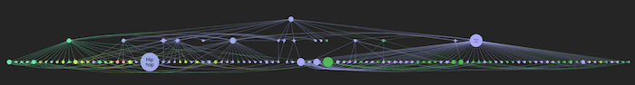
Here’s what happens when we load it into our visualization application:

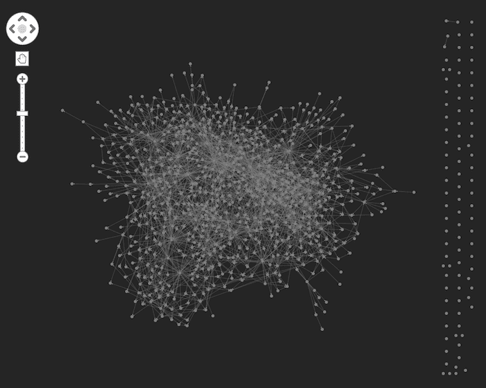
Yikes. This graph is a bit chaotic.

I’ve opted for a dark background and started with all nodes set to be the same light gray color. As expected, the main “component” in the graph is very well-connected. The organic layout immediately draws attention to the “singleton” nodes on the far right of the chart. These are likely to be data quality issues caused by a number of genres not having origin or derivative genres assigned to them in DBpedia. We’ll automatically filter these out so they don’t distract us from our core network.

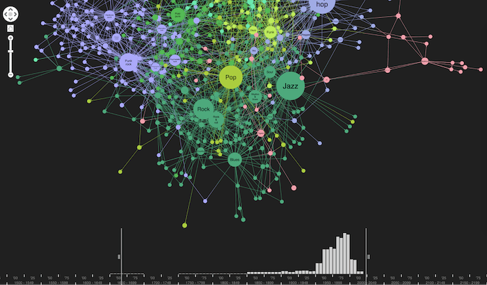
Let’s apply our built-in advanced social network analysis algorithms to size nodes depending on each genre’s overall influence.

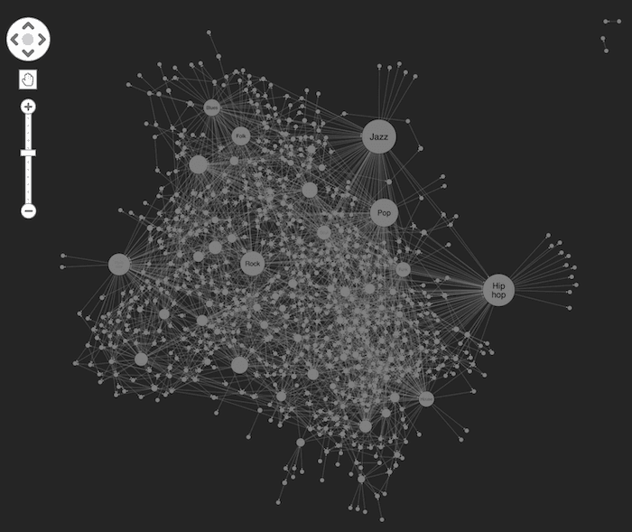
We’re starting to get a stronger feel for the network structure, but the chart is looking a little… well… boring. Let’s liven things up.

With our graph visualization toolkits, virtually everything on the chart can be styled however you like.

The most obvious attributes to inform our visual style are those included in the data source. I could, for example, color by each decade. However as we’re looking to spot patterns in our DBpedia knowledge graph data, I’m interested to see how our clustering function handles this tightly-connected network.

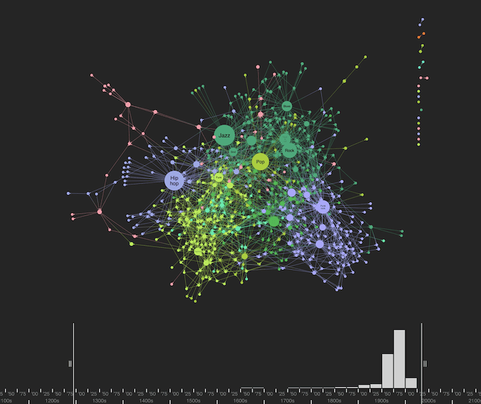
Clustering uses community detection routines to take an educated guess on the genres that may be similar. The links and direction of those links help to determine the “cluster” membership of each of the genres. Running clusters, applying a unique color to each cluster, and matching the node color on the link using our gradients function gives us this:

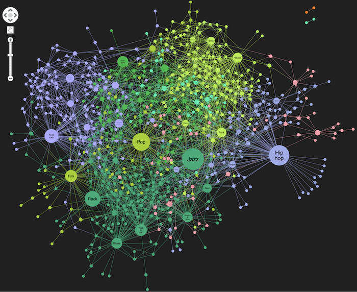
My intuition tells me the graph has been clustered pretty effectively. We see jazz, soul and rhythmn & blues clustered together.

Even so, each node can have a huge number of parents and children, which is why we see such a dense concentration of nodes.

Fortunately, our graph visualization toolkits have many other features to help in this scenario, including advanced network filtering, grouping similar nodes using combos and using the time bar to focus on specific time periods.

Let’s use the time bar to filter our knowledge graph visualization and look at music genres created in the 1970s only.

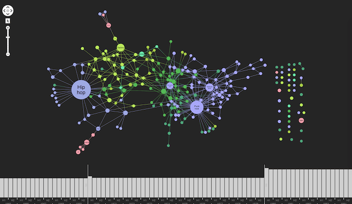
It was a very creative time for music. Much of today’s music derives from genres that emerged during that period – hip hop, punk rock, post-punk, etc. In this view, we can clearly see the impact of post-punk in the 1970s, which influenced or drew influence from, a network of other rock genres.

Let’s look at the most recently-created music genres:

I must admit I’ve never heard of “Wonky” before.

We can also see more obscure genres as singletons at the edge of the graph: psychedelic folk, doom metal, cadence-lypso, etc.

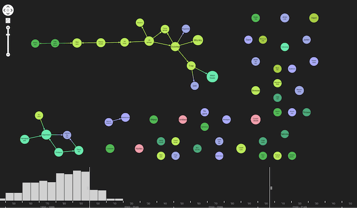
Using a sequential layout, we can track the influence of genres through the decades. Let’s see what happens when we click on Acid House:

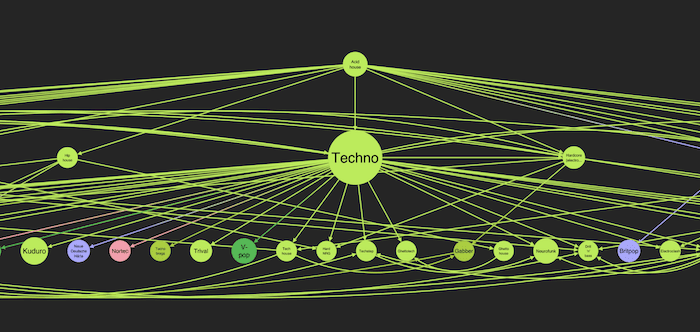
And drum & bass:

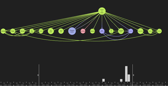
And finally, ska:

The nodes on the first level were directly influenced by the original genre. Further down we can see genres influenced by their children, and so on. Clicking these nodes takes our exploration further, working through a world of music.

Create your own knowledge graph

DBpedia is a goldmine of knowledge, available for you to explore – whether for fun, or to derive meaningful information. We’ve used it here to illustrate how easy it is to visualize a knowledge graph and make sense of the data.

For more details, check out our downloadable resources, contact our experts or request a free trial today.